Climate Feedbacks Explained, with Pie

The Rate of Change: September 23, 2019

A Pie Puzzle

Here’s a puzzle that might not seem like it has anything to do with the climate. But it’s at the heart of reasoning about how climate feedbacks work.

Say someone gave you an entire pie. Then they gave you half a pie. And then a quarter of a pie, and then an eighth of a pie, and so on, to infinity. At every step, you get half as much pie as you got before. How much pie would you end up with in the end?

At the heart of this puzzle is the remarkable realization that you can add up an infinite number of diminishing pieces and yet end up with a finite whole. It turns that all those infinitely many slices will add up to two full pies.

Mathematically, we can sum up this pie puzzle like this:

In math-speak, we’d say that this infinite series converges to a finite sum.

What does this have to do with Earth’s climate?

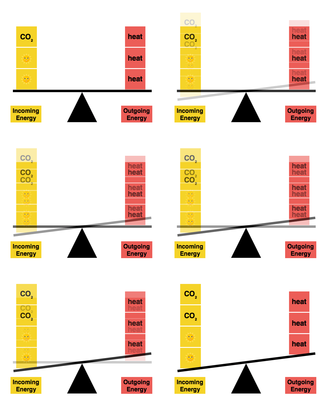
Earth’s temperature arises from a balance between the energy that we absorb and the energy that we radiate into space as heat. Because carbon dioxide is a heat-trapping gas, every unit of carbon dioxide that we emit tips the scales of Earth’s energy balance.

Adding CO2 tips the scales of Earth’s energy balance.

We’re currently out of balance, and are still tipping the scales further. This means that the Earth absorbs more energy than it can radiate away to space. This forces the Earth to warm up.

As the Earth warms, it’ll gradually start to radiate more heat into space. In the future, the Earth will find itself in a new energy balance, one where it has settled in to a warmer temperature.

Over time, the Earth will settle into a new, warmer energy balance.

Here’s a simple way to visualize this process, using Nicky Case’s feedback loop simulator.

You can press play and experiment with this for yourself. Pushing the up arrow emits carbon dioxide. Pushing the down arrow is equivalent to sucking CO₂ back from the air, either through natural or technological processes. The key takeaway is that the level of carbon dioxide in the air determines our eventual temperature rise.

In the previous newsletter and accompanying interactive, we came up with a number for this temperature rise. This is called the climate sensitivity, and it’s the answer to the question: how much does the temperature rise when you double CO₂ levels?

By balancing Earth’s energy budget, we estimated that a CO₂ doubling would cause a temperature shift of 1.1°C (about 2°F). However, climate scientists predict a much larger temperature shift of somewhere between 1.5 to 4.5°C (roughly 3-8°F).

So where did we go wrong?

Going around in circles

The reason our answer was too small is that we neglected all of the feedback loops in Earth’s climate system. For example, here’s a climate model that includes a process known as the water vapor feedback. (Interactive version here.)

Notice that adding a single unit of CO₂ now has a larger effect than before.

For every direct increase in temperature due to carbon dioxide’s greenhouse effect, there’s also an indirect increase from the cycle shown above. It works like this. As the temperature rises, more water evaporates. Water vapor is a greenhouse gas, so this extra water vapor traps more heat, and so the temperature rises further, which adds even more water vapor in the air, and so the cycle continues. This spiraling cycle is an amplifying feedback loop.

It’s worth remembering that even though water vapor is a greenhouse gas, turning on your lawn sprinkler won’t warm the planet. That’s because each drop of water that evaporates in your lawn will fall back down as rain in 9 to 10 days. The amount of water vapor in the air is limited by Earth’s average temperature, so any more that we try to add will eventually just fall back out as rain.

But as carbon dioxide warms the planet, evaporation ramps up. Unlike with your lawn sprinkler, in a warmer world there really is more water vapor in the air, and this water vapor further amplifies the initial warming.

So water vapor is a temperature multiplier.

Through the water vapor feedback cycle, the warming effect of carbon dioxide is roughly doubled. It’s as if every time that you raised the temperature on your thermostat by one degree, someone walked in to the room and set it a degree higher.

This is why feedbacks matter. They amplify change. They multiply the warming effect of carbon dioxide, and thereby shift climate change from being a cause for concern into becoming an all out emergency.

Climate Jargon: Things that directly alter Earth’s temperature by creating an energy imbalance are known as ‘forcings’. For example, an increase in the Sun’s brightness, or a volcano spewing sunlight-dimming ash are both possible types of forcings. In contrast, feedbacks act indirectly, by amplifying or diminishing the effect of a forcing. So water vapor is a feedback and not a forcing.

A Hidden Puzzle

But there’s a puzzle lurking within these loops.

If you think about it, doesn’t it seem like there’s no end to this feedback cycle? What prevents this process from spiraling out of control? And if this feedback loop will loop forever, doesn’t that mean that there’s no end to the warming?

ARE WE DOOMED?

OK, deep breaths. <inhale> <exhale>

To solve this puzzle, we need to take a closer look at how feedback loops work.

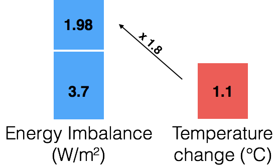
Say that we eventually double the carbon dioxide in Earth’s atmosphere. Climate scientists tell us that this will add 3.7 W/m² to Earth’s energy imbalance. Last week, we discovered that this will directly lead to about 1.1°C of warming.

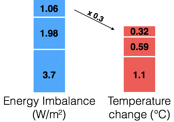
So every time we add an energy imbalance to the pile on the left, we can multiply it by 0.3 to get a temperature increase on the right.

But the warming is just getting started. For every degree that the temperature rises, climate scientists tell us that the water vapor feedback cycle will add 1.8 W/m² to our energy imbalance. So we can multiply the pile on the right by 1.8, and get the additional energy imbalance caused by one loop of the water vapor feedback cycle.

But wait! This additional energy imbalance will now cause its own rise in temperature. So once again, we multiply the blue box on top by 0.3.

And once again, this new temperature rise will add a little more to our energy imbalance. So we multiply the red box on top by 1.8.

Which, in turn, causes a further temperature rise. Maybe you see where this is going…

The cycle continues, repeating forever. With every loop, the red and blue piles grow a little bit taller.

As the feedback loop keeps looping, it looks a little like this:

The feedback factor tells you the effect of going around a feedback loop once. As the animation above shows, each loop contributes a factor of 1.8 times 0.3 (= 0.54, or about half) to the overall temperature change. In other words, every loop contributes about half the temperature change of the previous loop. Or, in the cartoon picture above, each new red block is about half the size of the block below it.

What does this remind you of? We started off with about one degree of warming. The water vapor feedback loop tacks on another half a degree of warming. Then it adds half of that. And half of that, and so on…

The water vapor feedback loop is the pie puzzle in disguise!

Just as we ended up with two pies, this feedback process amplifies one degree of warming into two degrees.

We can do a bit better than this. The gain of a feedback loop is the overall amount by which it multiplies the original effect. It turns out there’s a simple relationship between the feedback factor of a loop (its effect after one cycle) and its gain (its cumulative effect after all the cycles).

Here’s a chart that shows how the gain depends on the feedback factor.

A graph of the gain of a feedback loop (its cumulative effect after all the cycles) plotted versus its feedback factor (its effect after one cycle). Notice that as the feedback factor approaches 1, the gain blows up. This graph is from Gerard Roe’s paper Feedbacks, Timescales,and Seeing Red.

And here’s the formula for this graph.

Since the feedback factor of the water vapor loop was 1.8 ⨉ 0.3 = 0.54, plugging this into the formula tells us that its gain is 2.17. The water vapor feedback loop converts 1 degree of warming into ~2.2 degrees of warming.

In the pie puzzle, each slice of pie was smaller than the last, and this is what allowed us to reach a finite sum. Similarly, each loop of the feedback cycle makes a diminishing contribution to the overall temperature gain.

This is the solution to the loop puzzle — it’s the reason why we don’t end up with a runaway process that spirals out of control every time we have a feedback loop. An infinite series can converge to a finite sum.

The numberphiles among you may recognize the gain formula as the formula for the sum of a geometric series. If f represents the feedback factor due to one loop, then the gain due to all cycles of a feedback loop is given by the infinite sum 1 + f + f² + f³ + …, where each term in the series represents one more cycle of the feedback loop. Just like in the pie puzzle, each additional term contributes a diminishing amount to the overall sum. So this is a convergent sum (so long as the feedback factor f is less than 1), and the solution is that the total gain is 1 / (1 - f).

Loopology

There are essentially two kinds of feedback loops. Those with a positive feedback factor amplify changes, just like the water vapor cycle. Let’s call these amplifying feedback loops. (You can see from the graph above that a positive feedback factor implies a gain that’s bigger than 1.)

And then there are those with a negative feedback factor. Let’s call these regulating feedback loops, because they diminish the original change. (The graph above shows us that a negative feedback factor implies a gain that’s less than 1.) A classic example of a regulating feedback loop is a thermostat — when the room gets too hot, the thermostat switches off the heat, which cools the room back down.

Earth’s climate system is a complicated mix of amplifying and regulating feedback loops. So the picture looks more like this.

That’s quite a mess! (And even this is a massive simplification.)

It turns out that there’s one really nice feature of these complicated feedback loops. You can simply add together the feedback factors for each loop to get the feedback factor for their combined effect. And climate scientists have painstakingly estimated the feedback factors for each of these different loops.

The graph below shows a summary of these estimates. The column to the right is the sum of all the factors — that’s the number we’re after.

A graph from Gerard Roe’s paper Feedbacks, Timescales, and Seeing Red, compiling together different estimates of various climate feedback factors.

While the water vapor and lapse rate feedback cycles (the first two columns) individually have large uncertainties, it turns out if you consider them together (the third column) you can estimate them more accurately. Most of the uncertainty comes from estimating the feedback factor for clouds (the fifth column), which are notoriously difficult to model.

Adding all this together, you end up with a total feedback factor of about 0.6, with a considerable margin of error around that value.

Plugging 0.6 into our formula for the gain, this tells us that all these feedback loops together have a combined amplification effect (i.e. gain) of 1 / (1 - 0.6) = 2.5

So we can finally revise our estimate of the climate sensitivity. At first, we calculated that a doubling of carbon dioxide would lead to 1.1°C of warming. By taking these feedbacks into account, this number gets multiplied by 2.5, putting our revised prediction for Earth’s climate sensitivity at 2.75°C (which is within the range of accepted answers, if a bit on the low side).

So we’ve just seen how climate feedback loops amplify Earth’s climate sensitivity, and magnify climate change into a much bigger problem. In a coming newsletter, we’ll take a look at how these feedbacks also amplify uncertainty, and make it harder for us to predict the future.

---

References

This post was largely inspired by the article Feedbacks, Timescales, and Seeing Red by Gerard Roe, which was very helpful for me in understanding how feedback loops work. Any errors in understanding are entirely my fault.

This is the fourth part in a series of explainers on climate science. Part 1 and part 2 explore the idea of Earth’s energy balance, and part 3 builds on this idea to predict Earth’s climate sensitivity. This essay improves the climate sensitivity estimate from part 3 by incorporating climate feedbacks.

If you’re interested in learning more about the basics of climate science, I recommend David Archer's online lectures and textbook (he also has a Coursera course that covers similar material).

Don’t be out of the loop!

If you’re reading this on the substack website, or someone forwarded this essay to you as an email, you can stay in the loop (sorry!) with new posts by subscribing below.

If you’re already a subscriber, thanks! You’re amazing. If you like what you’re reading, maybe consider recommending this newsletter to a friend? It really helps get the word out.

The email header image is based on the Warning Stripes illustration by Alexander Radtke. The pie image is modified from Vecteezy.